2.1 Stress At A Point
2.1.1 Stresses on Rotated Planes – 3D
Suppose that we know the stress state of the soil on a particular plane, and we wish to determine the stress state on a different, rotated plane. This problem is equivalent to a transformation of the coordinate system. The components of the Cauchy stress tensor in the rotated coordinate space, \(\sigma_{ij}^{'}\), can be determined from the stress components in the reference state, \(\sigma_{ij}\), using the rotation matrix \(a\) with components \(a_{ij}\). Note that in soil mechanics, we often represent the shear stress components (i.e., the off-diagonal elements of the stress tensor) as \(\tau_{ij}\) instead of \(\sigma_{ij}\). Furthermore, the prime in \(\sigma'\) usually denotes effective stress, but is used here to denote stresses in a rotated coordinate system.
$$\sigma' = a \sigma a^T$$In matrix form:
\[\left[ \begin{matrix} \sigma _{11}^{'} & \sigma _{12}^{'} & \sigma _{13}^{'} \\ \sigma _{21}^{'} & \sigma _{22}^{'} & \sigma _{23}^{'} \\ \sigma _{31}^{'} & \sigma _{32}^{'} & \sigma _{33}^{'} \\ \end{matrix} \right]=\left[ \begin{matrix} {{a}_{11}} & {{a}_{12}} & {{a}_{13}} \\ {{a}_{21}} & {{a}_{22}} & {{a}_{23}} \\ {{a}_{31}} & {{a}_{32}} & {{a}_{33}} \\ \end{matrix} \right]\left[ \begin{matrix} \sigma _{11}^{{}} & \sigma _{12}^{{}} & \sigma _{13}^{{}} \\ \sigma _{21}^{{}} & \sigma _{22}^{{}} & \sigma _{23}^{{}} \\ \sigma _{31}^{{}} & \sigma _{32}^{{}} & \sigma _{33}^{{}} \\ \end{matrix} \right]\left[ \begin{matrix} {{a}_{11}} & {{a}_{21}} & {{a}_{31}} \\ {{a}_{12}} & {{a}_{22}} & {{a}_{32}} \\ {{a}_{13}} & {{a}_{23}} & {{a}_{33}} \\ \end{matrix} \right]\]
Figure 2.1.1. Stresses in a reference coordinate system (axes \(x_1\), \(x_2\), \(x_3\)), and rotated coordinate system (axes \(x_1'\), \(x_2'\), \(x_3'\)). https://upload.wikimedia.org/wikipedia/commons/thumb/7/76/Stress_transformation_3D.svg/2000px-Stress_transformation_3D.svg.png
Try it yourself
Note: The \(a\) matrix must be orthogonal (i.e., the axes in the rotated coordinate system must form 90 degree angles with each other)
| 2 | 0 | 0 |
| 0 | 1 | 0 |
| 0 | 0 | 1 |
Directly computing components of the \(a\) matrix is not always convenient. If you prefer, you may specify the rotation angles about the \(x_1\), \(x_2\), and \(x_3\) axes (\(\alpha\), \(\beta\), and \(\gamma\), respectively) below to set the \(a\) matrix.
\(\alpha\)deg
\(\beta\)deg
\(\gamma\)deg
2.1.2 Stresses on Rotated Planes – 2D
In soil mechanics, we often simplify three-dimensional stress conditions to two dimensions. The Mohr Circle is a very common tool used to interpret soil stress states, and it is inherently a two-dimensional representation of stresses. We should therefore consider rotation of stresses in two dimensions. Figure 2.1.2 defines the terms of the rotation tensor, \(a_{ij}\), in a manner that is consistent with the three-dimensional procedure in Figure 1.
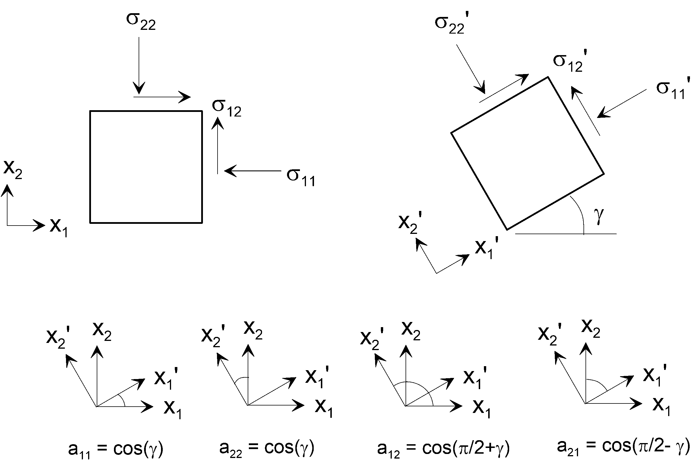
Figure 2.1.2. Two dimensional coordinate system rotation (note rotation is about the \(x_3\) axis by angle \(\gamma\)).
The rotated stress state can therefore be defined as follows: \[\left[ \begin{matrix} \sigma _{11}^{'} & \sigma _{12}^{'} \\ \sigma _{21}^{'} & \sigma _{22}^{'} \\ \end{matrix} \right]=\left[ \begin{matrix} \cos (\gamma ) & -\sin (\gamma ) \\ \sin (\gamma ) & \cos (\gamma ) \\ \end{matrix} \right]\left[ \begin{matrix} {{\sigma }_{11}} & {{\sigma }_{12}} \\ {{\sigma }_{21}} & {{\sigma }_{22}} \\ \end{matrix} \right]\left[ \begin{matrix} \cos (\gamma ) & \sin (\gamma ) \\ -\sin (\gamma ) & \cos (\gamma ) \\ \end{matrix} \right]\]
Expanding out the matrix algebra results in the following expressions for the rotated stresses: \[\begin{align} & \sigma _{11}^{'}={{\sigma }_{11}}-{{\sigma }_{12}}\sin (2\gamma )-{{\sin }^{2}}(\gamma )\left( {{\sigma }_{11}}-{{\sigma }_{22}} \right) \\ & \sigma _{22}^{'}={{\sigma }_{22}}+{{\sigma }_{12}}\sin (2\gamma )+{{\sin }^{2}}(\gamma )\left( {{\sigma }_{11}}-{{\sigma }_{22}} \right) \\ & \sigma _{12}^{'}={{\sigma }_{12}}\cos (2\gamma )+\frac{\sin (2\gamma )}{2}\left( {{\sigma }_{11}}-{{\sigma }_{22}} \right) \\ \end{align}\]
Try it yourself
deg
| 2 | 0 |
| 0 | 1 |
2.1.3 Graphical Solution for 2D: Pole Method
A graphical solution to the two-dimensional stress state on a plane inclined at any angle can be solved using the Mohr Circle. The steps are as follows:1. Plot stress state and draw Mohr Circle
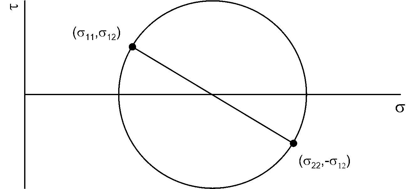
Figure 2.1.3a. Graphical solution of stresses on inclined plane: Step 1.
2. Draw line from (\(\sigma_{22},\sigma_{12}\)) in a direction perpendicular to the line of action of \(\sigma_{22}\). We assume here that \(\sigma_{22}\) acts vertically as illustrated in Fig. 2.1.2.

Figure 2.1.3b. Graphical solution of stresses on inclined plane: Step 2.
3. Draw line from (\(\sigma_{11},\sigma_{12}\)) in a direction perpendicular to the line of action of \(\sigma_{11}\).
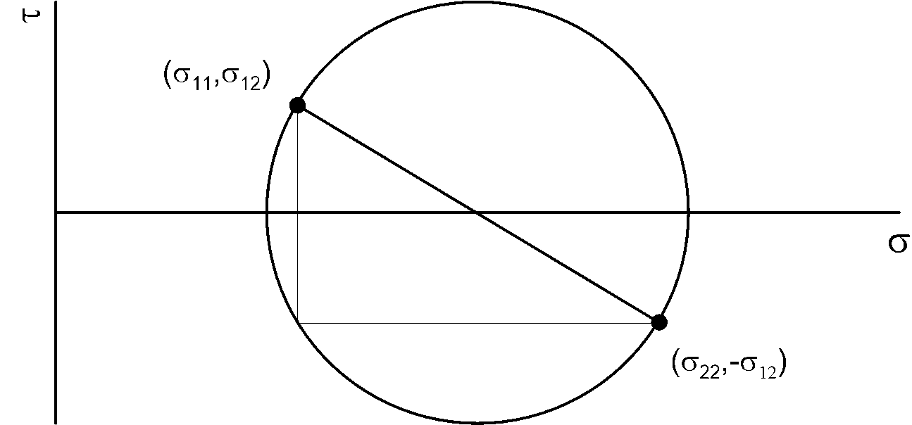
Figure 2.1.3c. Graphical solution of stresses on inclined plane: Step 3.
4. The intersection of the lines from Step 2 and 3 is called the "pole". The pole is a unique point on the Mohr circle because the stress state along a plane inclined at any angle \(\theta\) is defined by the intersection of the Mohr circle with a line drawn from the pole at an angle \(\theta\).
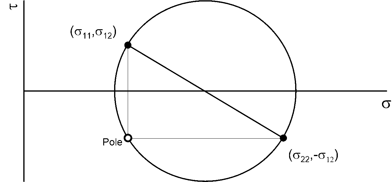
Figure 2.1.3d. Graphical solution of stresses on inclined plane: Step 4.
5. Draw a line angled at \(\theta\) from horizontal and \(\theta\) from vertical. The intersection of these lines with the Mohr circle defines the state of stress.
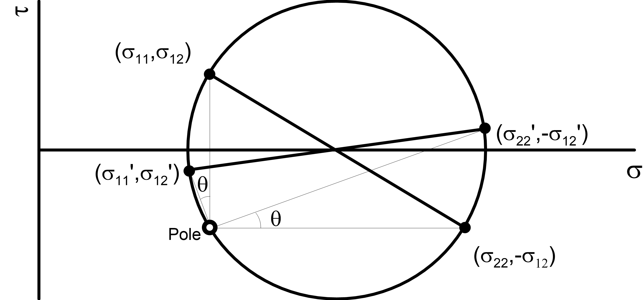
Figure 2.1.3e. Graphical solution of stresses on inclined plane: Step 5.
You may notice that we are using \(\theta\) to define the angle when we use the pole method, while we use \(\gamma\) to define the angle when we used the rotation matrix in the previous section. There is a good reason for this. \(\theta\) is an angle measured relative to the specific coordinate system under consideration, while \(\gamma\) is a change of angle from a reference plane to a rotated plane. Say, for example, that we know the stress condition for an element on planes that lie at angles \(\theta_1\) from horizontal and vertical, and we wish to find stresses on different planes rotated at angles \(\theta_2\) from horizontal and vertical. In this case, \(\gamma\) = \(\theta_2\) - \(\theta_1\). When finding the pole, it is important to draw the lines perpendicular to the line of action \(\sigma_{22}\) and \(\sigma_{11}\) in steps 2 and 3, respectively.
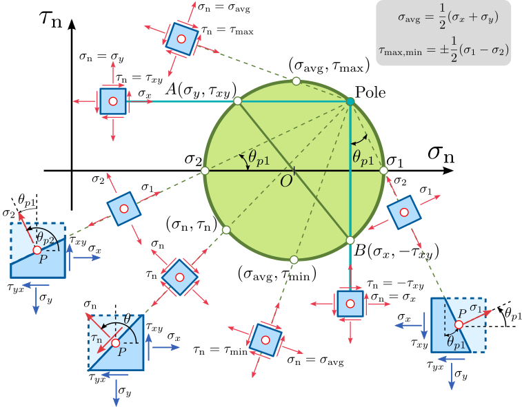
Figure 2.1.4. Mohr's circle for plane stress and plane strain conditions (Pole approach).
https://upload.wikimedia.org/wikipedia/commons/thumb/b/bd/Mohr_Circle_plane_stress_%28pole%29.svg/757px-Mohr_Circle_plane_stress_%28pole%29.svg.png